Local Influence Approaches On AUC

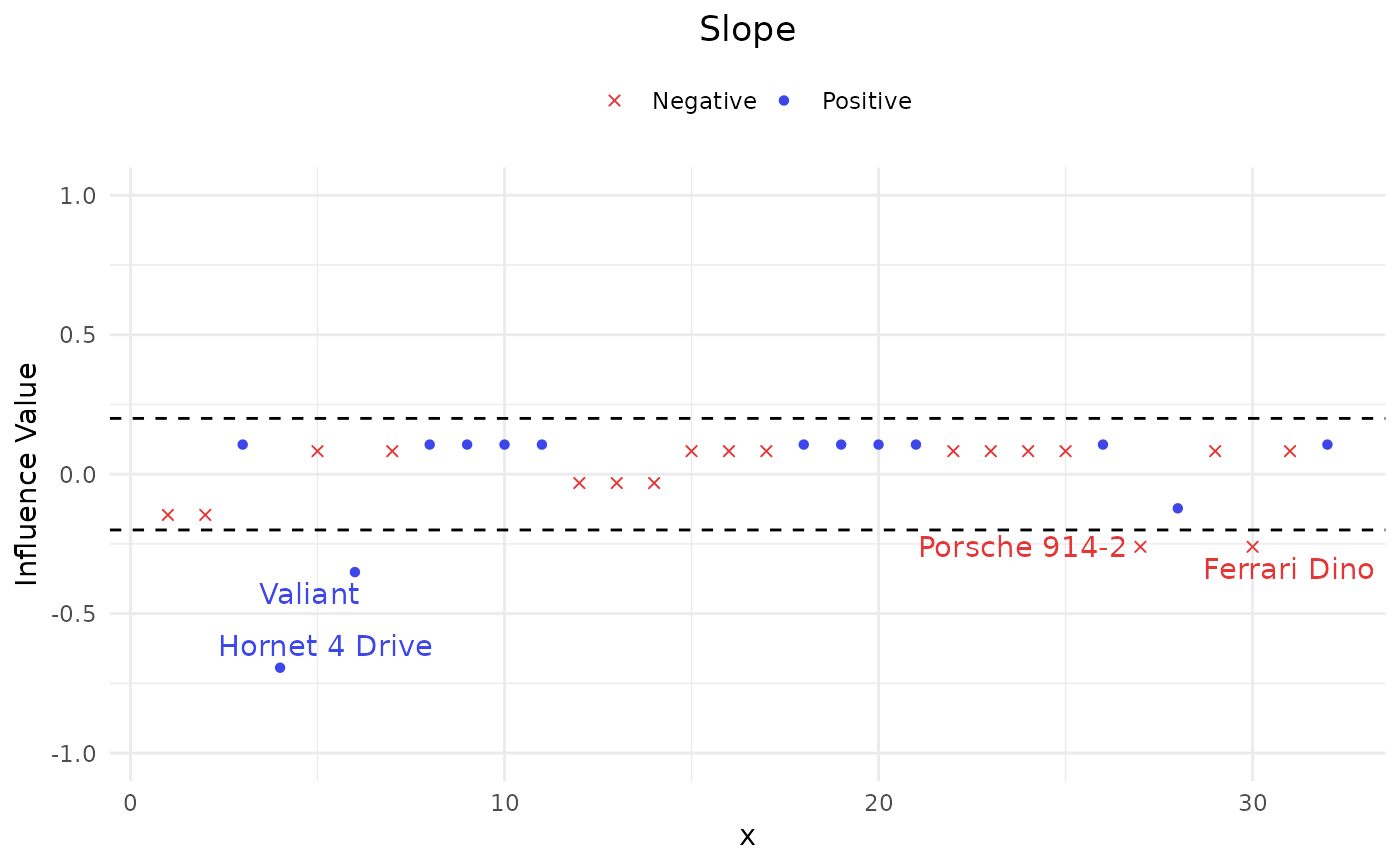
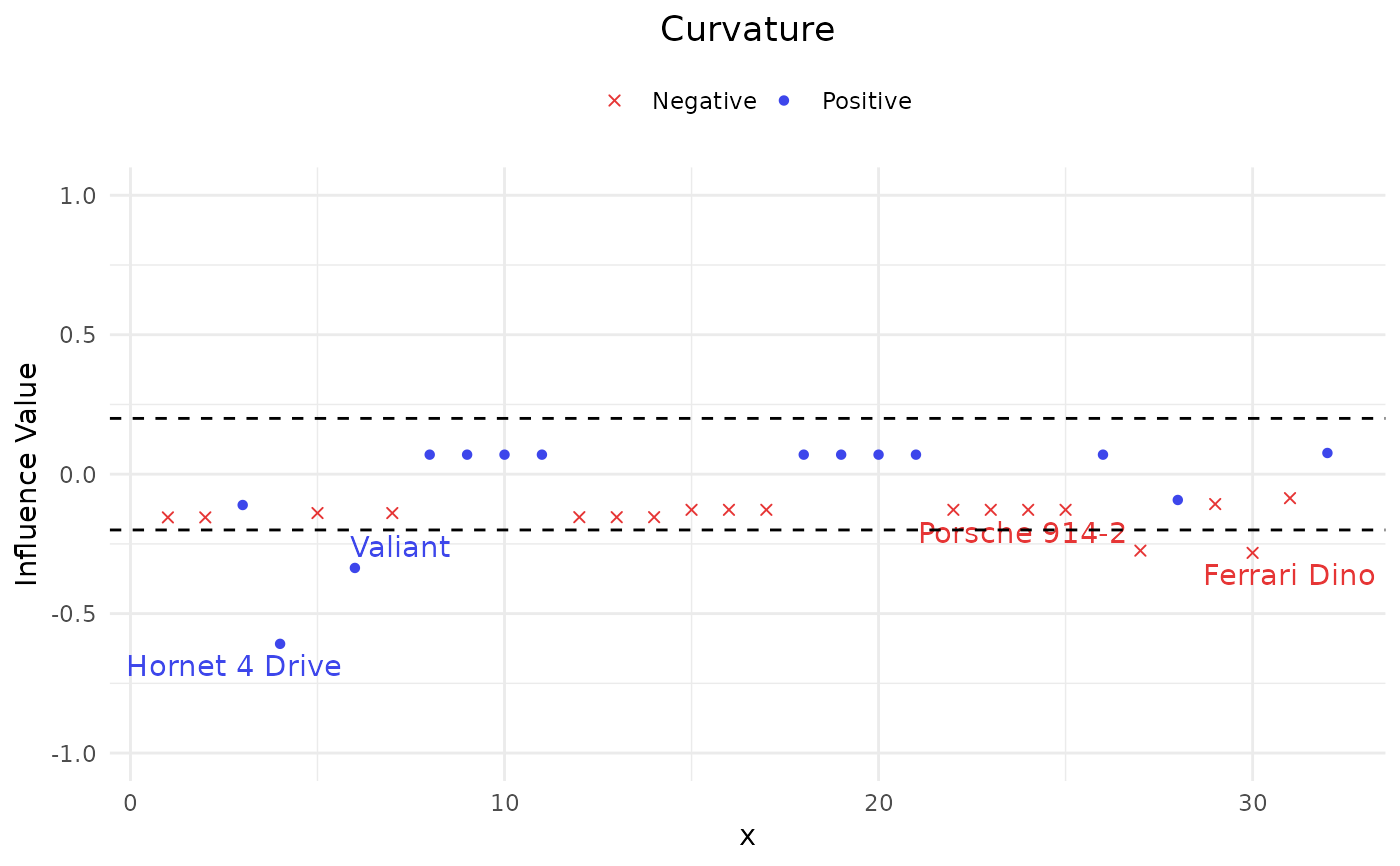
Apply local influence approaches in terms of slope and curvature on the AUC to quantify the impacts of all observations simultaneously.

LAUC(score, binary, threshold = 0.2, name = NULL)

Arguments

score: A vector containing the predictions (continuous scores) assigned by classifiers; Must be numeric.
binary: A vector containing the true class labels 1: positive and 0: negative. Must have the same dimensions as 'score.'
threshold: A numeric value determining the threshold to distinguish influential observations from normal ones; Must lie between 0 and 1; Defaults to 0.2.
name: A vector comprising the appellations for observations; Must have the same dimensions as 'score.'

Value

A list of objects including (1) `output`: a list of results with `AUC` (numeric), `Slope` (a list of dataframes) and `Curvature` (a list of dataframes)); (2) `rdata`: a dataframe of essential results for visualization (3) `threshold`: a used numeric value to distinguish influential observations from normal ones.

Details

The influence functions on the AUC focus on the deletion diagnostics; however, such approaches may encounter the masking effect. Rather than dealing with single observations once at a time, local influence methods address this issue by finding the weighted direction of all observations accompanied by the greatest (magnitude) slope and curvature. From the explicit formula based on the slope, local influence methods may face the imbalanced data effect. To thoroughly investigate the potential observation in binary classification, we suggest end-users to apply ICLC and IAUC as well. For a complete discussion of these functions, please see the reference.

References

Ke, B. S., Chiang, A. J., & Chang, Y. C. I. (2018). Influence Analysis for the Area Under the Receiver Operating Characteristic Curve. Journal of biopharmaceutical statistics, 28(4), 722-734.

Author

Bo-Shiang Ke and Yuan-chin Ivan Chang

Examples

library(ROCR)
data("ROCR.simple")
# print out LAUC results directly
LAUC(ROCR.simple$predictions,ROCR.simple$labels)
#> output is: 
#> $AUC
#> [1] 0.8341875
#> 
#> $Slope
#> $Slope$Pos
#>      Index  influence
#> [1,]    29 -0.2854024
#> [2,]    86 -0.2886361
#> [3,]    93 -0.2013255
#> [4,]   145 -0.2207279
#> [5,]   178 -0.2854024
#> 
#> $Slope$Neg
#>      Index  influence
#> [1,]    25 -0.2379357
#> [2,]    77 -0.2185334
#> [3,]   108 -0.2379357
#> [4,]   193 -0.2411695
#> 
#> 
#> $Curvature
#> $Curvature$Pos
#>      Index  influence
#> [1,]    86 -0.2090887
#> [2,]   178 -0.2746311
#> 
#> $Curvature$Neg
#>      Index influence
#> 
#> 

data(mtcars)
glmfit <- glm(vs ~ wt + disp, family = binomial, data = mtcars)
prob <- as.vector(predict(glmfit, newdata = mtcars, type = "response"))
output <- LAUC(prob, mtcars$vs, name = rownames(mtcars))
# Show results
print(output)
#> output is: 
#> $AUC
#> [1] 0.9484127
#> 
#> $Slope
#> $Slope$Pos
#>                Index  influence
#> Hornet 4 Drive     4 -0.6939810
#> Valiant            6 -0.3510727
#> 
#> $Slope$Neg
#>               Index  influence
#> Porsche 914-2    27 -0.2603563
#> Ferrari Dino     30 -0.2603563
#> 
#> 
#> $Curvature
#> $Curvature$Pos
#>                Index  influence
#> Hornet 4 Drive     4 -0.6083615
#> Valiant            6 -0.3362089
#> 
#> $Curvature$Neg
#>               Index  influence
#> Porsche 914-2    27 -0.2741215
#> Ferrari Dino     30 -0.2821815
#> 
#> 
# Visualize results
plot(output)